
Transit Scheduling 101: Developing A Runtime
Runtime (n) - The time required for the transit vehicle to travel from one end of the line to the other. We'll take a deeper look at runtimes in this installment of Transit Scheduling 101!

By now, we’ve covered the two chunks of time that make a transit vehicle’s trip; layover and runtime.
Layover (n). - Time scheduled into a transit route for the vehicle to recover any time lost in the last lap and start the next lap on time. This also offers an opportunity for the driver to take a break to prepare the best version of themselves for the next trip.
Runtime (n) - The time required for the transit vehicle to travel from one end of the line to the other.
Sufficient layover ensures the transit vehicle and its driver can recover time from any unexpected delays and be prepared to start the next trip on time. My baseline assumption for layover is at least 15% of runtime, meaning that a bus that has been driving for 30 minutes is owed at least a 5 minute break, often more depending on how the scheduling math lands. Note that layover is supposed to accommodate unexpected delays, like special event traffic near the high school, or a fare dispute that held the bus up at a stop. These one-off delays are just life behind the wheel.

However, if the bus is consistently getting to its layover late, and the bus driver is consistently expected to sacrifice their layover to keep the bus on schedule, you probably should take a look at your runtimes.
⏱️The Structure of a Runtime
Recall this route with a 24 minute runtime (one way).
From this schedule, we learn that it takes 24 minutes for the bus to travel between the bus station and Walmart. We also learn that it takes 8 minutes to get from the bus station to the high school, 6 minutes to get from the high school to the grocery store, 6 minutes to get from there to the office park, and 4 more minutes to get to the Walmart. These timepoint to timepoint runtimes are the domain of the transit scheduler.
Timepoint (n) - Designated stops along a route where vehicles are scheduled to arrive and depart at specific times. Stops between timepoints are not assigned exact arrival or departure times, but are bound by the timepoints before and after them. Timepoints are typically located at major stops, transfer hubs, terminals, and other places where the bus can hold for time without being an obstruction. Timepoints provide control points for operators and form the basis of published timetables
Developing runtimes at the timepoint level makes it easier to adjust the schedule as travel times push and pull over time.
⌛Developing a Runtime
One of the easiest traps that you can fall into when developing a brand new runtime is to spin your wheels trying to develop the perfect runtime.
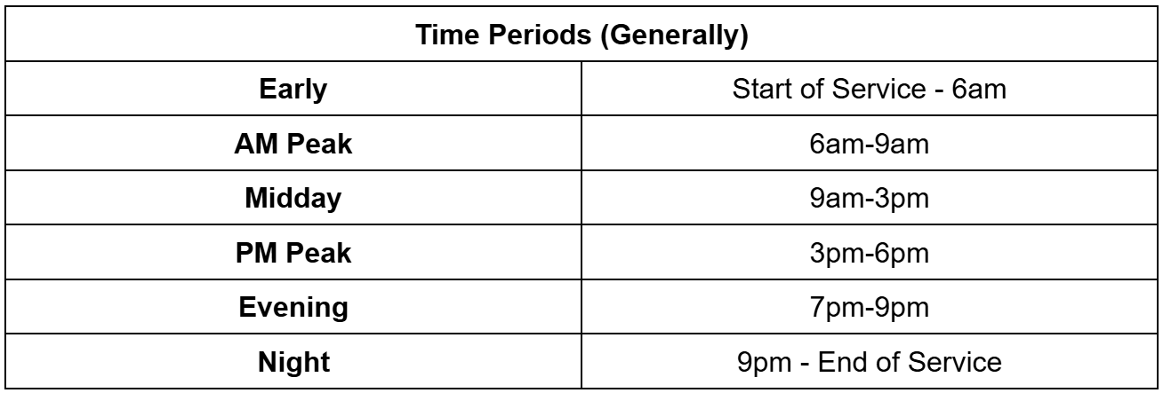
The runtime is not attempting to perfectly model how long each trip in the schedule takes, it’s meant to capture how long it takes the average bus driver to complete the trip. Since runtime often changes throughout the day, runtimes are typically broken out by time period, with specific runtimes applied to specific times of day. Here are the time periods I typically start with when building a runtime from scratch.
While the number of time periods can fluctuate depending on the local context, it is again important to remember that the runtime is not attempting to perfectly model how long each trip in the schedule takes.
In my time as a scheduling consultant, I’ve occasionally encountered schedules with hourly time bands, meaning runtimes change every hour. Please don’t do this. Scheduling relies on repeating patterns, and this ensures patterns will rarely repeat. At higher frequencies, it also just short of guarantees you will have scheduled and unscheduled bus bunching at the edges of time bands, particularly if the runtimes and frequencies change drastically from band to band. When we explore blocking in a future article, we’ll dive into why
When you’re developing a runtime, it’s less important that your initial runtime is perfect, and more important that you adjust the runtime as you operate the route and learn where the sticky points are. Even if the published runtime hasn’t changed in years, I guarantee the real world runtime has. Runtimes are not static. Traffic will build. Activity centers will shift along the route and throughout the city. Ridership will ebb and flow, impacting how much time is spent boarding passengers. A “perfect” runtime that never changes is less helpful than a good enough runtime that is updated regularly.
With that in mind, here are three, simple and effective ways to develop good enough runtimes to be further refined as you learn how the route operates. All of these approaches use publicly available tools and information.
🖥️Method #1: Using the National Transit Database
Most (all?) transit authorities in the United States are required to report metrics about their service to the Federal Transit Administration National Transit Database. The Service annual dataset includes the total revenue miles and revenue hours operated by a transit authority, amongst other figures. Dividing the revenue miles by the revenue hours offers a crude estimate for the speed of the service.
Note that revenue hours include layover time when the bus isn’t moving, so these speeds are a bit faster than the actual vehicle travel speed.
If you’re developing a runtime for a new route in an area where there is already transit service, this crude runtime can serve as a jumping off point for developing a runtime for a new route in its service area. Here are a handful of transit authorities and their service speed.1
Based on this, if you were developing a runtime for a 6.7 mile route in Kansas City, how much runtime would it require? (Here’s a speed-distance-time calculator if you’re not into quick math)
How much runtime would the same route require in Chicago?
This approach provides a high level estimate of the end to end runtime, to be subdivided into timepoint to timepoint runtimes. Admittedly, this is the most crude of the methods for developing a runtime, but this approach, paired with appropriate layover, produces the framework for a good enough schedule to be updated and revised as the service is operated and real world runtimes are observed.
🗺️Method #2: Using Google Maps
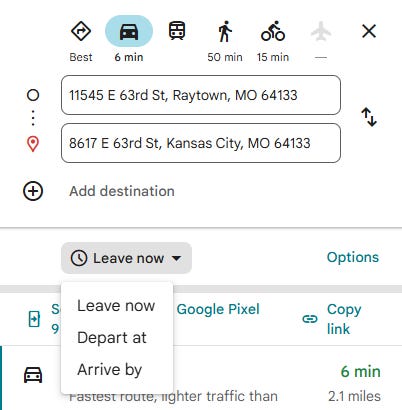
On February 8th, 2005, a software debuted that would revolutionize transportation planning forever, bringing route planning and travel time estimation into an accessible, comprehensible platform. That software? Google Maps! In 2025, 20 years after its launch, Google Maps is still guiding transportation planning decisions the world over. Let’s use this tool, plus some estimates about bus stop spacing and dwell times, to develop a runtime for the proposed, 6.7 mile route, shown below.
This route connects major destinations throughout Raytown, MO, an immediate suburb of Kansas City, MO. If you plug the timepoints from this route into Google Maps like so, you can view the distances and travel times between timepoints. From this information you can get travel speeds between the timepoints, as well as the travel time and speed for the entire route. In a car, this 6.7 mile route would take 19 minutes, at an average speed of 21.2 mph.
To translate these car travel times and speeds into bus travel times and speeds, we need to add in the expected time that the bus spends at bus stops, as well as the time required to accelerate and decelerate from those stops. Fortunately, this can be estimated relatively easily via some basic assumptions.
Assumptions #1: How many stops are on the route.
Assumption #2: How long does the bus typically spend serving each stop
Assumption #3: What percentage of the stops will the bus stop at on a typical trip
Assuming stops are spaced every 1/4 mile, we find that this route has 28 stops. If we assume each stop takes 20 seconds, and 50% of the stops will be stopped at on a typical trip, we should add 5 minutes to the overall travel time to account for stops. This increases the end to end travel time from 19 minutes to 24 minutes, resulting in an average speed of 17 mph2.
These assumptions should be tailored to the local context. For example, if this route was operating in Chicago, I would assume an 1/8 mile stop spacing, with something like 75% of the stops being stopped at on a typical trip, resulting in 55 stops and 14 minutes of additional travel time.
While this example created a single runtime, this process works for developing time period specific runtimes as well. To do this, simply adjust the “Depart at” time in Google Maps, and repeat the process with the new Google travel times.
🚌Method #3: Find a Bus and Drive the Route
Even in this era of modern technology solutions, sometimes there is still merit to doing things the old fashioned way. If you don’t want to parse through NTD or Google Maps data, then the simplest approach to developing a runtime might be to just hop behind the wheel of a bus and drive the proposed route several times with a stopwatch, timing how long it takes you to travel from timepoint to timepoint. If you employ this method, take your time, and make sure to make several simulated stops along the route to reflect real world travel conditions. Many transit authorities require new bus drivers to undergo several weeks of training runs before they’re cleared to start driving in revenue service with passengers onboard. While these training runs typically follow existing routes, sending drivers in training to drive new or proposed routes puts this required, behind the wheel training time to more productive use, while ensuring runtimes don’t skew fast from testing runs performed by experienced bus drivers that are more comfortable behind the wheel.
I was once told I “drove the hell out of this bus” by a passenger, so I might be part of the problem. In my defense, compressed natural gas buses haul.
Even if this approach is not used to develop a runtime, It can be a valuable tool for testing the sanity of a route before the schedule goes live. Beyond timing, getting out and driving the proposed route provides an opportunity to check the specifics of the alignment to ensure timepoints are in reasonable locations, and turns can be reasonably accomplished by the vehicles (and drivers) assigned to the route. There are few things more embarrassing than starting a new service, and having to reroute it immediately because a turn that looked doable on Google Maps was absolutely NOT doable.
Now, armed with three approaches to developing runtimes, you should be more than comfortable developing runtimes for a transit route. If you do find yourself developing a runtime and spinning your wheels in the future, remember, perfect is the enemy of good. Give it your best attempt, and refine the runtime as the route operates.
📚 Buy me a Book 💚
Thanks for reading! If you enjoy my writing and want to support it in a small but meaningful way, consider buying me a book from my Bookshop.org wishlist. It’s the books that I want to read, but have not quite pulled the trigger yet!
directly operated (DO), motorbus (MB)